The question of TIME has puzzled humanity for millennia. What is it? Does it flow like a river or is it a simple dimension that can be transversed even traveling back to observe the past? Aristotle was one of the first to ponder what is TIME. His account of TIME in Physics IV.10-14, is where he argued that “now” is not part of TIME for it was neither the past nor the future – it divides the past and the future.
We are all familiar with three dimensions since we can move up, down, left, or right in our world. But there is a fourth dimension that’s just as important – TIME. We’re always moving forward through TIME as we understand it, yet it’s just as much a dimension as any of the spatial ones we are familiar with. We definitely live in a four-dimensional Universe which is described by the fabric of spacetime, or a 3+1 dimensional Universe. We cannot separate TIME from our 3-D world for they are all interdependent. Nothing would exist if there were no TIME. In order to completely describe an event in spacetime, you also need to know more than just where it occurs, but also when it occurs.
Hermann Minkowski (1864-1909) actually took one of those giant steps for mankind when he realized, mathematically, of course, that moving through TIME behaves exactly as moving through space does, with the exception that with two additional multiplicative factors: c, the speed of light in a vacuum, and i, the imaginary number √(-1). After completing his derivation of spacetime for the first time, Minkowski concluded that space by itself, and time by itself, were doomed to fade away into mere shadows, and only a union of the two will preserve an independent reality. What all of this means to us in studying markets is highly relevant.
When it comes to markets and analysis, without TIME, we are truly lost. The world of Newtonianism with absolute space and absolute TIME dooms us also in analysis. Even as we would move through the Universe, we would experience changes in how space and TIME pass. When we look at market activity, we cannot separate TIME from the 3-D analysis of market behavior. For this reason, we have explored TIME for it cannot be separated from analysis either.
CYCLE INVERSIONS & SUPERPOSITION
There MUST also be a Cycle Inversion to keep the complexity and to hide reality from those who walk through like like a horse with blinkers on. Cycles exist both on a fixed level of time as well as a dynamic level within TIME, which we will explain later herein – Longitudinal & Transverse. Now, this may all sound like sophistry so you can have it both ways. A target in TIME where we would normally expect say a cycle low inverts and produces a high, but on the same target in TIME. We call this a Cycle Inversion for it is the product of global interference for we are all connected. Look how events in 2014 in Ukraine have infected the entire world economy.
This is also why politics is doomed. No politicians can alter the global trend of the economy no matter what they promise. The world we live in is not a straight line. Although we travel a straight line ourselves between birth and our inevitable death, along the way we experience ups and downs – the good times and the bad. There is a cycle to absolutely everything from our brainwaves to a woman’s menstrual cycle. Consequently, a Cycle Inversion is where the target in TIME is valid, but the event is a high or a low may not always be predictable because of the interconnectivity of everything around the world.
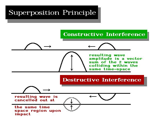
The Superposition Principle is a very important occurrence within the cyclical movement of everything. In physics and systems theory, the Superposition Principle states that, for all linear systems, the net response caused by two or more stimuli is the sum of the responses that would have been caused by each stimulus individually. That is the foundation of our Timing Array bringing together 72 independent models. This principle applies to cyclical behavior within a single market, which we can qualify as simply a linear system without interfacing it with all other markets that introduce a nonlinear system of super-complexity.
 The best example so you can see this interesting phenomenon is to study wave motion in the ocean. We I was young, growing up in New Jersey, I would go to the beach. I had a couple of uncles who live on the beach back then. I was fascinated by the waves as they hit the shore. I would count between each wave and notice there was a regularity to wave structure. But then I would notice one wave would be larger than all the ones before and after. I found that curious.
 Throughout history even from ancient times, sailors have told stories of some mythical sea monster – the Kraken (Cracken). This emerged from what we now understand are that rogue wave I would see as a kid sitting on the beach. The Japanese created a famous picture of it called the “Great Wave.” Today, we know that they exist and they are what we now call the “Rogue Wave” that appears out of nowhere. That famous Japanese print, known as the “Great Wave”, does not portray a tsunami caused by an earthquake. The Great Wave pictures what its title denotes, simply a large okinami, which actually means a “wave of the open sea.” Until 1995, these “Great Waves” or “Rogue Waves” were known only from stories and legends of sailors. The 1972 movie Poseidon Adventure depicts an ocean liner which turned upside down by one of these waves.
 These legends of massive waves that drag ships to their doom have often been attributed to giant monsters of something supernatural are simply wave motions that take place also in economics. In reality, they can be simply explained as “cyclical convergences” whereby numerous cyclical waves combine together and produce an abnormally “giant” or “large” wave that causes the amplitude of the individual waves to blend together producing a huge abnormal event – like the Great Depression or the Great Recession of 2007-2010. This is a Constructive Inference that produces these giant waves in the ocean as well as in economics.
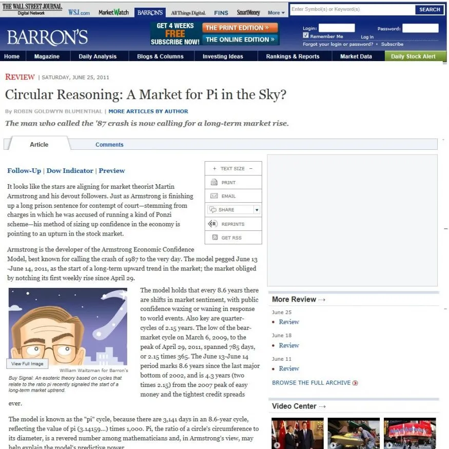
When we forecast that the market would rise to new record highs in 2010, and even Barron’s had to write about our forecast they, like most in the mainstream press, thought it was laughable. All it proved is that mainstream media lives in this linear world that cannot ever see the change in trend ahead because they simply do not understand the cyclical nature of everything in this universe. On the day of the low in 1987, our model forecasted that the low would hold and we would make new highs by 1989. Many thought we were crazy back then as well. Once more, the world refuses to understand that everything is cyclical.
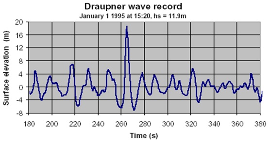
 This mysterious legendary Great Wave, or Rogue Wave, was finally confirmed in 1995. That is when the first measurement of such a wave took place. It is now known as the Draupner Wave. It struck the Draupner oil platform in the North Sea off the coast of Norway on January 1st, 1995. This provided the first opportunity to actually measure such a wave carried out by Engineer Paul Taylor. The platform survived this event, but the wave, measured with lasers, was 84 feet high (25.6 meters) in a sea where the average wave only measured was 39 feet in height (12 meters). This provides us with a real-world chart of exactly what a Superposition Principle is all about – how a Constructive Inference produces extraordinary events.
In economics, this is the convergence of economic trends from a global perspective that combine to produce major economic upheavals. The first confirmed Global Economic Depression was that of the Panic of 1857. Yet throughout recorded history, there were many such events one could attribute to these Rogue Economic Waves dating back to when all the countries defaulted on the Greek Central Bank known as the Temple of Delos. A Stella survives recording all the government defaults during the period. That was the first such sovereign default that took place during the 4th century BC when ten out of thirteen Greek municipalities in the Attic Maritime Association defaulted on loans from the Delos Temple of Apollo.
It is this Superposition Principle that accounts for economic events such as the Great Depression. It is the convergence of many cycles that suddenly all align to combine and produce a catastrophic event that nobody can predict by simple human opinion.
Understanding TIME

The thing you have to understand about market movement is that we can forecast two types of events depending on the data being employed. What are turning points, this is typically a common question. The timing arrays do NOT forecast a specific event be it a high or a low, it forecasts TURNING POINTS, which can be measured generally on the intraday event or on a closing event. As illustrated here, sometimes the highest closing and the intraday can be as much as 4 units of time apart in separation. So that applies on a fractal basis from the Daily to Yearly level.
Keep in mind that market movement is extremely complex. You should approach this subject ONLY if you can observe everything around you and notice how things are connected. If you are expecting just to BUY and SELL without comprehending how everything functions, then this is not the model for you. What you are being presented with here is the tools to allow you to listen to what the markets are telling you. Oh, they do speak to us. They are by no means random walking like some drunk through the park late at night. Nothing takes place which is disconnected from the whole.
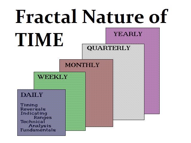
The first lesson to grasp here is that markets are indeed FRACTAL in nature. The patterns replicate through all levels of time. We designed this model so you can differentiate short-term counter-trend moves from real-world changes in trend. So we look for actual changes in a trend that must be confirmed from Monthly to Yearly Models. The Daily level offers the greatest “noise” whereby we witness shifts bullish and bearish all the time. The Weekly level offers more of a counter-trend move which might be sustainable for a few months before resuming the long-term trend.
How to Use the Forecasting Arrays
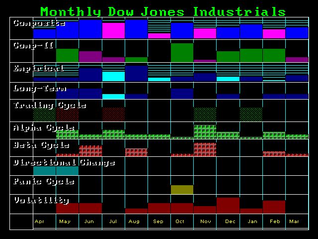
The Forecasting Arrays are a great visual display generated by our computer models. These arrays are a composite of 72 models in total which cover trading patterns, volatility, Directional Changes, Panic Cycles, and of course the turning points from an immediate to long-term basis. There are two primary technological methods being incorporated here. First, we have turning points that are cyclical based. Then we have Pattern Recognition which is reflected in the Direction Change. Our Forecasting Arrays are the sum of all models. As such, they cannot be reverse-engineered since they are by no means based upon a single model or formula.
The first thing you should understand is that the charting is proportional, and not explicit. For example, let’s say that January had 30 hits from 72 models. That would be the highest bar. Then January passes and May show up as the highest bar when it was previously half that of January when previously charted. The bars are plotted on a relative basis to the time frame selected. So if the highest bar has 15 hits within that 12th unit of time, it will be at the top. As time moves forward and a new target enters the window with 25 hits, it will now appear at the top and the bar with 15 hits will appear as if it diminished. So the charting is RELATIVE and not explicit.
The MOST IMPORTANT bar to pay attention to for TURNING POINTS will be the top bar labeled COMPOSITE. This is where we have the sum of all models. You can be declining in price as the bars are rising. They do not reflect direction, but changes in trend. Looking at the above example, a decline into May would imply a May low with June then showing a change in that trend which may be a bounce. Likewise, if the market was rallying into May, then June would imply a decline. This is a change in the trend we call Turning Points which can be intraday or on a closing basis.
ALPHA & BETA Cycles
The Alpha Cycle is derived ONLY from market highs. The Beta Cycle is derived from ONLY just price lows. Then the cycles are determined on each basis EXCLUSIVELY. While ideally, one would expect these to forecast like events, that does not always pan out in that fashion. Once more, there are 72 independent models in these Arrays, and they are all then combined into the top line of the Array.
CYCLICAL TIMING MODELS
There are two primary types of cyclical wave formations – the Transverse Wave and the Longitudinal Wave structure containing patterns. The computer models are further divided between fixed cycles and cyclical activity determined entirely by the computer.

The EMPIRICAL (hard-wired) transverse frequencies of a fixed duration are displayed in a separate line both short and long-term frequencies. Then there is the far more complex dynamic longitudinal wave frequencies which fluctuate in duration. These are entirely ascertained by the computer on its own without predetermining the frequencies. This is displayed in the second row from the top listed as Composite for here this line reflects ALL the various cycle frequencies the computer discovers without limitation. These are the two primary types of cyclical activity.
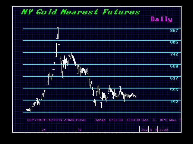
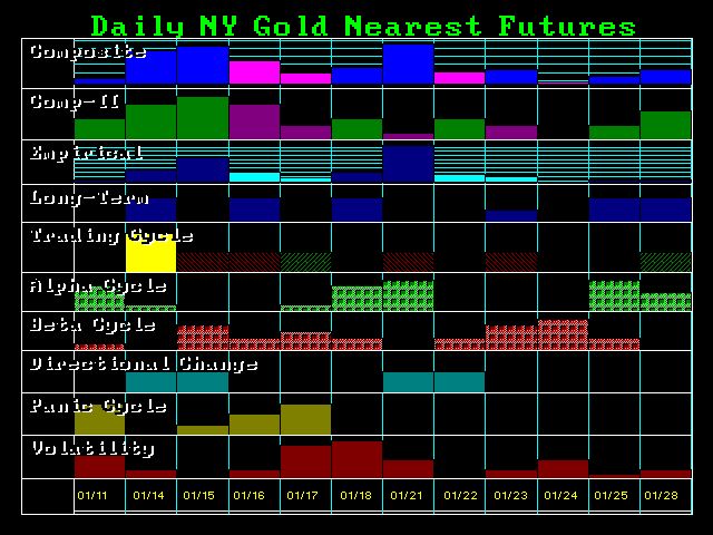
Gold Daily January 1980
Figure #1
The top line is the Composite, which is the sum of the cyclical models below including both Transverse and Longitudinal based cyclical timing models. As stated above, this is the primary line to watch for this reflects the most important turning points which can be high or low. You obviously know the difference as you are moving into that target date.
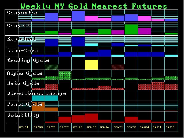
Pictured here in Figure #1 is an Array for gold in January 1980 at the major high compiled January 9, 1980. We can see that this picked January 21 as the high. There were two sets of back-to-back Directional Change targets. The first was 5 days BEFORE the high and clearly marked the breakout to the upside the second caught the actual high on the 21st of January. That morning, Gold opened up the limit at $875 on the spot closing at $850 after falling to $831. It had been just $597 at the low the week of January 7 and rallied about $300 into January 21 st. We can see that the top Composite picked the 21st as did the Empirical timing model which is Transverse in design.
The Directional Change can be by itself a very fascinating tool. The Directional Change can at times be the beginning of a breakout to a new trading level (major thrust) in one direction in which the market is making a break to a new plateau in price movement up or down. However, at other times, Directional Changes can mark the high or low and the culmination of a trend. The Daily Array on gold pictured at the top showed two Directional Changes back to back which picked the major high in Gold during 1980.

Figure #2
Figure #3
The Directional Change can at times be the beginning of a breakout to a new trading level as was the case for the week of 11/02/2014 in the Dow. This was confirming that the Dow would take off to a new plateau in price movement.
Figure #4
Directional Changes can also mark the high or low and the culmination of a trend as illustrated at the top with the Daily gold for January 19080. Here in Figure #4 look at the weeks of 07/14/2014 and 12/22/2014. The Directional Change for the week of 07/14 was followed by a major turning point 2 weeks later both on the top Composite and the Long-Term, which produced the spike low. We see the same type of pattern where the Directional Change of 12/22 was preceded by the major turning point for 12/08 which was also the key spike low in Figure #3.
The week of 01/19/2015 produced the highest closing for that reaction with the intraday high the week before (Figure #2). Then the Dow fell into the intraday low two weeks later.
Figure #5
A Panic Cycle is a target that normally exceeds either one direction up or down forcefully, but it is also a target that can be an OUTSIDE REVERSAL either to the upside or downside (meaning it exceeds the previous session high and penetrates the low). Hence, a Panic Cycle can be a move either to the upside whereby it begins lower than the previous session and then exceeds the high, or an outside reversal to the downside whereby it begins strong exceeding the previous high and then penetrating the previous low. This differs from Volatility which can be measured in three primary different manners (see below). Here in Figure #5, we can see that gold broke out to the upside the week of February 8th in line with our Panic Cycle target for that week.
Figure #6
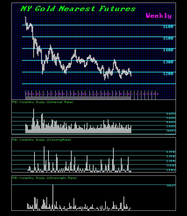
Volatility Models are dependent upon how you are measuring volatility. Do you define that as close to close, from last night’s close to the morning open, or do you measure volatility as the percentage movement that day between the high and the low? Illustrated above in Figure #6 we have plotted these three main types of volatility so you can see there is a huge difference. Obviously, the definition of volatility being plotted and forecast can be correct in one manner and a non-event in another. It all depends upon your definition.
There is overnight volatility reflected in the percentage movement from the previous session closing to the current session opening. Then there is intraday volatility measured by the distance between the high and low of the trading session. Then there is closing volatility from one session to the next. We can see that these three perspectives alone provide completely different forecasts.
Detailed Video Explanation of the Array
Here is a detailed explanation of the Forecasting Array.
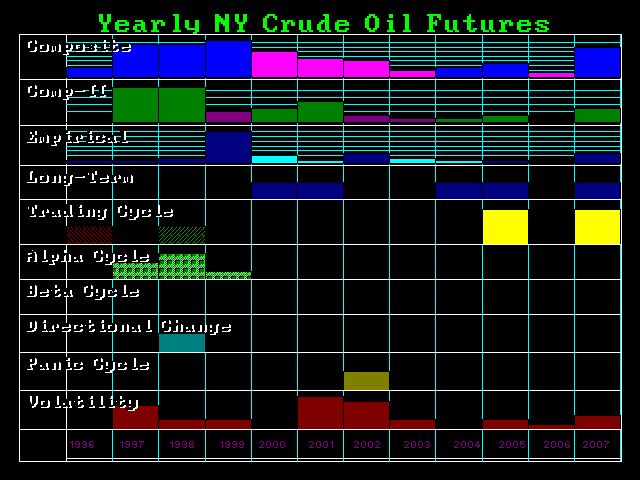
Detailed VIDEO on the Crude Array 1996
The Long-Term view perspective of the 1996 forecast for Crude oil into 2007
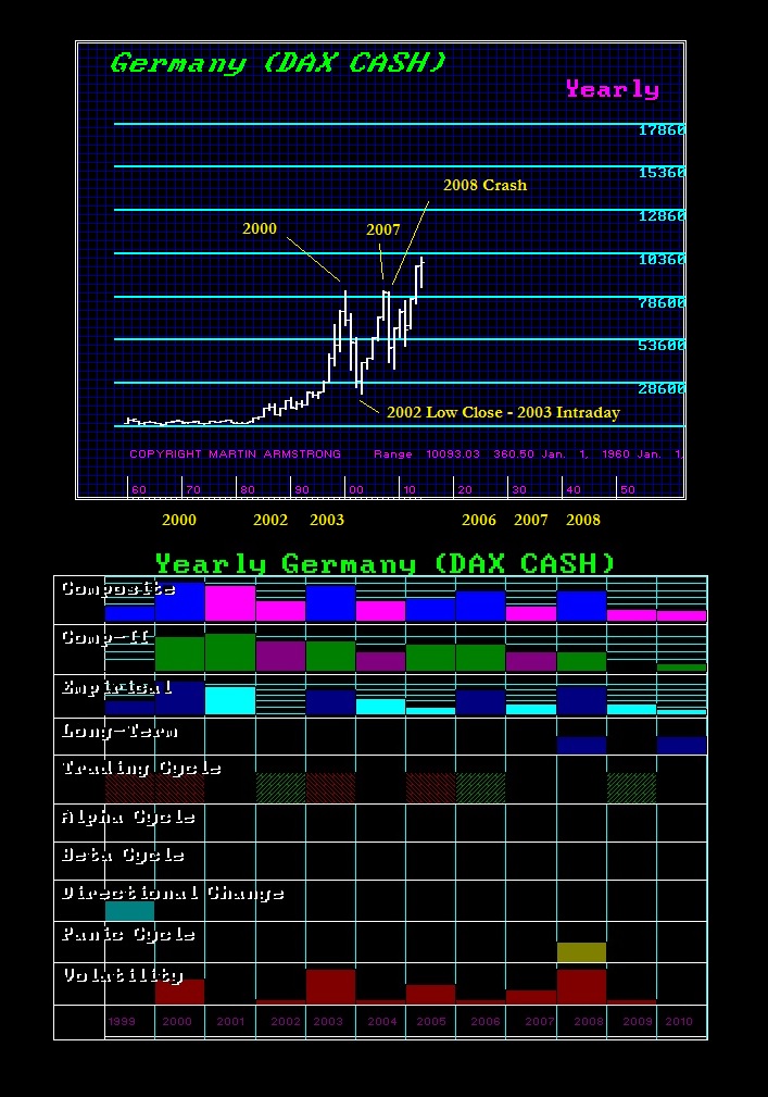
Here is the Yearly Array for the DAX we published in 1999. You can see that even on the Yearly Level, the computer did a fairly good job in picking the years for turning points.
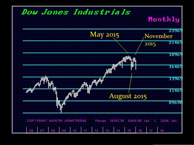
The May high in the Dow was on an intraday basis and this lined up with the Directional Change. The next target was August which provided the low, and October was the Panic to the Upside. November was favored as we moved closer to the people for the turning point whereas here that showed up at first on the Empirical level (longitudinal or fixed frequency).


![ezgif 5 014fc9ef71 An animated look at how spacetime responds as a mass moves through it helps showcase exactly how,... [+] qualitatively, it isn't merely a sheet of fabric but all of space itself gets curved by the presence and properties of the matter and energy within the Universe. Note that spacetime can only be described if we include not only the position of the massive object, but where that mass is located throughout time. Both instantaneous location and the past history of where that object was located determine the forces experienced by objects moving through the Universe.](https://blogs-images.forbes.com/startswithabang/files/2018/08/ezgif-5-014fc9ef71.gif?)

